Sky Atmosphere In XEngine

Note that this Project was written during my undergraduate studies. Some points may be incorrect.

Brief Introduction to UE’s Implementation

This project is based on the implementation of the unreal engine. I assume that you have a basic knowledge of volume rendering and will not go into detail about it. If you are interested, you can read my blog about Volume Rendering In Offline Rendering.
Here are some basic terms about the sky atmosphere rendering:

σa\sigma_{a}: absorption coefficient, the probability density that light is absorbed per unit distance traveled in the medium.
σs\sigma_{s}: scattering coefficient, the probability of an out-scattering event occurring per unit distance.
σt\sigma_{t}: attenuation coefficient, the sum of the absorption coefficient and the scattering coefficient, describes the combined effect of the absorption and out scattering.
σt=σa+σs\sigma_{t} = \sigma_{a} + \sigma_{s}
T(a,b)T(a,b): transmittance, the fraction of radiance that is transmitted between two points
T(a,b)=eabσt(h)dsT(a,b)=e^{-\int_{a}^{b}\sigma_{t}(h)\mathrm{d}s}
ϕu\phi_{u}: phase function, the angular distribution of scattered radiation at a point

Volume Rendering Euqation:
The lighting result at the point x from direct v equals the combination of single scattering and multi-scattering:

L(x,v)=L1(x,v)+Ln(x,v)L(x,v) = L_{1}(x,v) + L_{n}(x,v)

The single scattering result at point x from point p in direction v is the sum of the transmitted radiance reflected from the ground and the integration of the radiance from the view point to the ground or sky:

L1(x,p,v)=T(x,p)L0(p,v)+t=0pxσsT(x,xtv)T(xtv,xtv+tatmoli)ϕuEidtL_{1}(x,p,v) = T(x,p)L_{0}(p,v)+\int_{t=0}^{||p-x||}\sigma_{s}T(x,x-tv)T(x-tv,x-tv+t_{atmo}l_{i})\phi_{u}E_{i}\mathrm{d}t

N-bounce multi-scattering (LnL_{n}) integrate the GnG_{n} in the point along the view direction, where GnG_{n} is the integration of the Ln1L_{n-1} scattering result from the direction on the sphere. Multi-Scattering is difficult to calculate compared to Single-Scattering. There are many simplifications that are made in UE’s sky-atmosphere for multi-scattering, we will be introducing it later.

Ln(x,v)=t=0pxσs(x)T(x,xtv)Gn(xtv,v)dtL_{n}(x,v) = \int_{t=0}^{||p-x||}\sigma_{s}(x)T(x,x-tv)G_{n}(x-tv,-v)\mathrm{d}t
Gn(x,v)=ΩLn1(x,v)ϕudwG_{n}(x,v)=\int_{\Omega}L_{n-1}(x,-v)\phi_{u}\mathrm{d}w

Transmittance LUT

There are two important properties of beam transmittance. The first property is that the transmittance between two points is the same in both directions if the attenuation coefficient satisfies the directional symmetry σt(w)=σt(w)\sigma_{t}(w) = \sigma_{t}(-w) :

T(a,b)=T(b,a)T(a,b) = T(b,a)

Another important property, true in all media, is that transmittance is multiplicative along points on a ray:

T(a,b)=T(a,c)T(c,b)T(a,b) = T(a,c) T(c,b)

This property enables us to calculate the transmittance between any two points quickly by precalculating the transmittance between these two points and the boundary of the sky atmosphere:
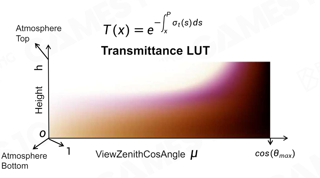
T(a,b)=T(a,boundnary)T(b,boundnary)T(a,b) = \frac{T(a,boundnary)} {T(b,boundnary)}
T(a,b)T(a,b) is a 3-dimensional function of the dimension x,y and z. We can convert this function to a 2-dimensional function of the view height and view zenith angle, since the earth is symmetric horizontally.

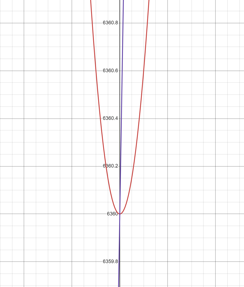
Transmittance lut’s u coordinate is view zenith cosine angle ranging from -1 to 1. In addition, the v coordinate is mapped to the view height ranging from the bottom radius to the top radius. Bruneton’s paper use a generic mapping, working for any atmosphere, but still providing an increased sampling rate near the horizon. In the following figure, the red curve represents Bruneton’s implementation, while the purple curve represents a linear interpolation.

We can get the world position and world direction from the view height and the view zenith angle mapped from the texture coordinates.

1
2
3
4
5
6
7
8
float2 UV = (PixPos) * SkyAtmosphere_TransmittanceLutSizeAndInvSize.zw;

float ViewHeight;
float ViewZenithCosAngle;
UvToLutTransmittanceParams(ViewHeight, ViewZenithCosAngle, UV);

float3 WorldPos = float3(0.0f, ViewHeight, 0);
float3 WorldDir = float3(0.0f, ViewZenithCosAngle,sqrt(1.0f - ViewZenithCosAngle * ViewZenithCosAngle));

The next step is to calculate optical depth. It is an intergal along the direction of view from the point of view to the boundary of the atmosphere:

τ(s)=0pσt(s)ds\tau(s)= -\int_{0}^{p} \sigma_{t}(s)ds

This equation is viewed as a ray marching from the view point to the boundary for coding:

1
2
3
4
5
6
7
8
9
10
11
float dt = tMax / SampleCount;
float3 OpticalDepth = 0.0f;
for (float SampleI = 0.0f; SampleI < SampleCount; SampleI += 1.0f)
{
t = tMax * (SampleI + DEFAULT_SAMPLE_OFFSET) / SampleCount;
float3 P = WorldPos + t * WorldDir;
MediumSampleRGB Medium = SampleMediumRGB(P);
const float3 SampleOpticalDepth = Medium.Extinction * dt;
OpticalDepth += SampleOpticalDepth;
}
return OpticalDepth;

The medium extinction contains two parts: mie extinction and rayleigh extinction, which is a expontial function of the view height:

σt(h)=σt_mi(h)+σt_rayleigh(h)\sigma_{t}(h) = \sigma_{t\_mi}(h) + \sigma_{t\_rayleigh}(h)

Participating media following the Rayleigh and Mie theories have an altitude density distribution of dt_mi(h)=eh8kmd_{t\_mi}(h) = e^{\frac{-h}{8km}} and dt_ray(h)=eh1.2kmd_{t\_ray}(h) = e^{\frac{-h}{1.2km}} , respectively.
Rayleigh participation media components have different coefficients, which results in a blue sky at noon and a red sky at dusk.
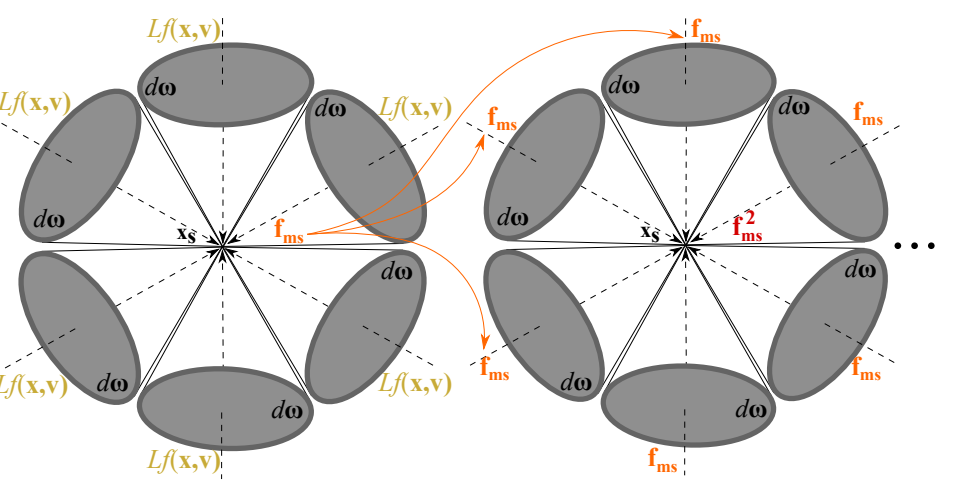
1
2
3
4
5
6
7
8
9
10
11
12
13
14
15
16
17
18
19
20
21
22
23
MediumSampleRGB SampleMediumRGB(in float3 WorldPos)
{
const float SampleHeight = max(0.0, (length(WorldPos) - Atmosphere_BottomRadiusKm));
const float DensityMie = exp(Atmosphere_MieDensityExpScale * SampleHeight);
const float DensityRay = exp(Atmosphere_RayleighDensityExpScale * SampleHeight);

MediumSampleRGB s;

s.ScatteringMie = DensityMie * Atmosphere_MieScattering.rgb;
s.AbsorptionMie = DensityMie * Atmosphere_MieAbsorption.rgb;
s.ExtinctionMie = DensityMie * Atmosphere_MieExtinction.rgb; // equals to ScatteringMie + AbsorptionMie

s.ScatteringRay = DensityRay * Atmosphere_RayleighScattering.rgb;
s.AbsorptionRay = 0.0f;
s.ExtinctionRay = s.ScatteringRay + s.AbsorptionRay;

s.Scattering = s.ScatteringMie + s.ScatteringRay;
s.Absorption = s.AbsorptionMie + s.AbsorptionRay;
s.Extinction = s.ExtinctionMie + s.ExtinctionRay;
s.Albedo = GetAlbedo(s.Scattering, s.Extinction);

return s;
}

Here is the transmittance LUT result. We ignore the ozone’s contribution, which results in the absence of the purple region in the LUT:

Multi-Scattering

As we mentioned above, it’s difficult to calculate the GnG_{n}, unreal engine makes two simplification for this part.
The first simplification is:

Scattering events with order greater or equal to 2 are executed using an isotropic phase function ϕu\phi_{u}

Gn(x,v)=ΩLn1(x,v)ϕudw14πΩLn1(x,v)dtG_{n}(x,v)=\int_{\Omega}L_{n-1}(x,-v)\phi_{u}\mathrm{d}w\approx \frac{1}{4\pi}\int_{\Omega}L_{n-1}(x,-v)\mathrm{d}t

The second simplification is:

All points within the neighborhood of the position we currently shade receive the same amount of second order scattered light

Ln1(x,v)=t=0pxσs(x)T(x,xtv)Gn1(xtv,v)dtGn1t=0pxσs(x)T(x,xtv)dtL_{n-1}(x,v) = \int_{t=0}^{||p-x||}\sigma_{s}(x)T(x,x-tv)G_{n-1}(x-tv,-v)\mathrm{d}t\approx G_{n-1}\int_{t=0}^{||p-x||}\sigma_{s}(x)T(x,x-tv)\mathrm{d}t

Combine these equation together, we get:

Gn(x,v)14πΩLn1(x,v)dw14πGn1Ωt=0pxσs(x)T(x,xtv)dtdwG_{n}(x,v)\approx \frac{1}{4\pi}\int_{\Omega}L_{n-1}(x,-v)\mathrm{d}w\approx \frac{1}{4\pi} G_{n-1}\int_{\Omega}\int_{t=0}^{||p-x||}\sigma_{s}(x)T(x,x-tv)\mathrm{d}t\mathrm{d}w

GnGn1=14πΩt=0pxσs(x)T(x,xtv)dtdw=14πΩfmsdw\frac{G_{n}}{G_{n-1}} = \frac{1}{4\pi}\int_{\Omega}\int_{t=0}^{||p-x||}\sigma_{s}(x)T(x,x-tv)\mathrm{d}t\mathrm{d}w = \frac{1}{4\pi}\int_{\Omega}f_{ms}\mathrm{d}w

fms=t=0pxσs(x)T(x,xtv)dtf_{ms}=\int_{t=0}^{||p-x||}\sigma_{s}(x)T(x,x-tv)\mathrm{d}t

Our next step is to precompute the 14πΩfmsdw\frac{1}{4\pi}\int_{\Omega}f_{ms}\mathrm{d}w value and store it in the two-dimensional LUT table.UE’s sky atmosphere has three different integration methods for different quality levels. The first implementation is to integrate the fmsf_{ms} on the uniform sphere, which is expensive and only used in case of high quality.The second one is to integrate fmsf_{ms} 8 times with the following ray direction:

What we employed in the xengine is the last approach: sample twice from the view direction and negative direction:

GnGn1=14πΩfmsdw=14π(fms(x,v)+fms(x,v))0.5\frac{G_{n}}{G_{n-1}}=\frac{1}{4\pi}\int_{\Omega}f_{ms}\mathrm{d}w=\frac{1}{4\pi}(f_{ms}(x,v) + f_{ms}(x,-v)) * 0.5

fms=t=0pxσs(x)T(x,xtv)dtf_{ms}=\int_{t=0}^{||p-x||}\sigma_{s}(x)T(x,x-tv)\mathrm{d}t
1
2
3
4
5
6
7
8
9
10
11
12
13
14
15
16
17
18
float dt = tMax / SampleCount;
float3 Throughput = 1.0f;

for (float SampleI = 0.0f; SampleI < SampleCount; SampleI += 1.0f)
{
t = tMax * (SampleI + DEFAULT_SAMPLE_OFFSET) / SampleCount;
float3 P = WorldPos + t * WorldDir;
float PHeight = length(P);

MediumSampleRGB Medium = SampleMediumRGB(P);
const float3 SampleOpticalDepth = Medium.Extinction * dt * 1.0f;
const float3 SampleTransmittance = exp(-SampleOpticalDepth);

MultiScatAs1 += Throughput * Medium.Scattering * 1.0f * dt;

Throughput *= SampleTransmittance;
}
OutMultiScatAs1=MultiScatAs1;

With fmsf_{ms}, we can precompute the multi-scattering result in arbitray rorder.

G2=G1fms=L114πfmsG_{2}=G_{1}f_{ms}=L_{1}\frac{1}{4\pi}f_{ms}
G3=G2fms=G114πfmsfms=L114πfms2G_{3}=G_{2}f_{ms}=G_{1}\frac{1}{4\pi}f_{ms}f_{ms}=L_{1}\frac{1}{4\pi}f_{ms}^{2}
Gn=L114πfmsn1G_{n}=L_{1}\frac{1}{4\pi}f_{ms}^{n-1}
Gn+Gn1+...+G1=L114π(fmsn1+fmsn2+...+1)=L114π(11fms)G_{n}+G_{n-1}+ ... +G_{1}=L_{1}\frac{1}{4\pi}(f_{ms}^{n-1} +f_{ms}^{n-2}+ ... +1)=L_{1}\frac{1}{4\pi}(\frac{1}{1-f_{ms}})

The single scattering result L1L_{1} is required to compute by the time of the fmsf_{ms} calculation.

1
2
3
4
5
6
7
8
9
10
11
12
13
14
15
16
17
18
19
float3 OutL_0, OutMultiScatAs1_0, OutL_1, OutMultiScatAs1_1;
ComputeScattedLightLuminanceAndMultiScatAs1in(
WorldPos, WorldDir, LightDir, OneIlluminance,
SkyAtmosphere_MultiScatteringSampleCount, OutL_0, OutMultiScatAs1_0);
ComputeScattedLightLuminanceAndMultiScatAs1in(
WorldPos, -WorldDir, LightDir, OneIlluminance,
SkyAtmosphere_MultiScatteringSampleCount, OutL_1, OutMultiScatAs1_1);

const float SphereSolidAngle = 4.0f * PI;
const float IsotropicPhase = 1.0f / SphereSolidAngle;

float3 IntegratedIlluminance = (SphereSolidAngle / 2.0f) * (OutL_0 + OutL_1);
float3 MultiScatAs1 = (1.0f / 2.0f) * (OutMultiScatAs1_0 + OutMultiScatAs1_1);
float3 InScatteredLuminance = IntegratedIlluminance * IsotropicPhase;

// For a serie, sum_{n=0}^{n=+inf} = 1 + r + r^2 + r^3 + ... + r^n = 1 / (1.0 - r)
const float3 R = MultiScatAs1;
const float3 SumOfAllMultiScatteringEventsContribution = 1.0f / (1.0f - R);
float3 L = InScatteredLuminance * SumOfAllMultiScatteringEventsContribution;

Sky-View LUT

With the precomputed transmittance LUT and the multi-scattering result, it’s enough to ray marhcing the sky atmosphere with a low number of samples:

L=0b(L1+σsGall)dtL = \int_{0}^{b}(L_{1} + \sigma_{s}G_{all})\mathrm{d}t

We can get the multi-scattering term GallG_{all} by looking up the LUT precomputed before.

1
float3 MultiScatteredLuminance0 = MultiScatteredLuminanceLutTexture.SampleLevel(gsamLinearClamp, MultiSactterUV, 0).rgb;

The remaining single scattering term is the integration along the view direction:

L=0b(Vis(p,v)T(p,v)(σs_mieϕmie+σs_rayϕray)+σsGall)dtL = \int_{0}^{b}(Vis(p,v)T(p,v)(\sigma_{s\_mie}\phi_{mie}+ \sigma_{s\_ray}\phi_{ray})+\sigma_{s}G_{all})\mathrm{d}t, where Vis is the shadow term in this position and the transmittance term is obtained from transmittance lut.
1
2
3
4
5
6
float3 TransmittanceToLight0 = TransmittanceLutTexture.SampleLevel(gsamLinearClamp, UV, 0).rgb;
float3 PhaseTimesScattering0 = Medium.ScatteringMie * MiePhaseValueLight0 + Medium.ScatteringRay * RayleighPhaseValueLight0;

float tPlanet0 = RaySphereIntersectNearest(P, Light0Dir, PlanetO + PLANET_RADIUS_OFFSET * UpVector, Atmosphere_BottomRadiusKm);
float PlanetShadow0 = tPlanet0 >= 0.0f ? 0.0f : 1.0f;
float3 S = Light0Illuminance * (PlanetShadow0 * TransmittanceToLight0 * PhaseTimesScattering0 + MultiScatteredLuminance0 * Medium.Scattering);

Another important term is the phase function term, which indicates the relative ratio of light lost in a particular direction after a scattering event. Here is the rayleigh phase function. The 316π\frac{3}{16\pi} coefficient serves as a normalisation factor, so that the integral over a unit sphere is 1:

ϕray(θ)=316π(1+cos2(θ))\phi_{ray}(\theta)=\frac{3}{16\pi}(1+cos^{2}(\theta))

We use the simpler Henyey-Greenstein phase function for mie scattering:

1
2
3
4
5
6
float HgPhase(float G, float CosTheta)
{
float Numer = 1.0f - G * G;
float Denom = 1.0f + G * G + 2.0f * G * CosTheta;
return Numer / (4.0f * PI * Denom * sqrt(Denom));
}

Latitude/Longtitude Texture

UE’s implementation renders the distant sky into a latitude/longtitude sky-view LUT texture in a low resolution and upscales the texture on the lighting pass.In order to better represent the high-frequency visual features toward the horizon, unreal engine applies a non-linear transformation to the latitude l when computing the texture coordinate v in [0,1] that will compress more texels near the horizon:

v=0.5+0.5sign(l)lπ/2v = 0.5 + 0.5 * sign(l) * \sqrt{\frac{|l|}{\pi/2}}
1
2
3
4
5
6
7
8
9
10
11
12
13
14
15
16
17
18
19
20
float Vhorizon = sqrt(ViewHeight * ViewHeight - BottomRadius * BottomRadius);
float CosBeta = Vhorizon / ViewHeight;
float Beta = acosFast4(CosBeta);
float ZenithHorizonAngle = PI - Beta;
float ViewZenithAngle = acosFast4(ViewZenithCosAngle);

if (!IntersectGround)
{
float Coord = ViewZenithAngle / ZenithHorizonAngle;
Coord = 1.0f - Coord;
Coord = sqrt(Coord);
Coord = 1.0f - Coord;
UV.y = Coord * 0.5f;
}
else
{
float Coord = (ViewZenithAngle - ZenithHorizonAngle) / Beta;
Coord = sqrt(Coord);
UV.y = Coord * 0.5f + 0.5f;
}

Combine Light

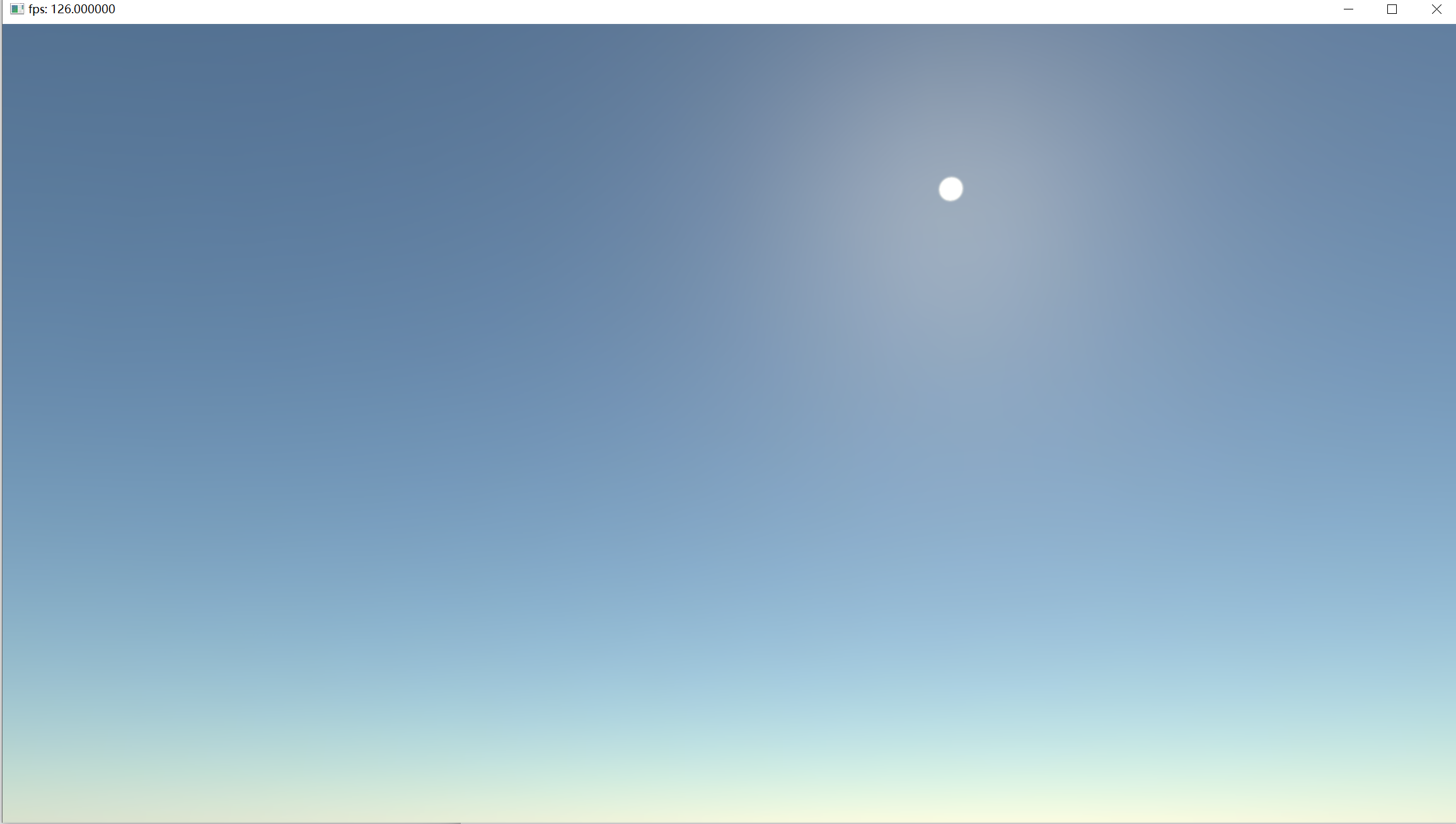
Sky-View LUT doesn’t calculate sun disk luminance, since it is high-frequency lighting, which should be computed at full resolution in the lighting pass based on the view direction and the light direction. The rest low-frequency part can be obtained by looking up the sky-view LUT directly. Below is the result of our implementation in XEngine.

sky atmosphere source code


Sky Atmosphere In XEngine
http://example.com/2024/05/05/Sky-Atmosphere-In-XEngine/
Author
Shawn Tang
Posted on
May 5, 2024
Licensed under